


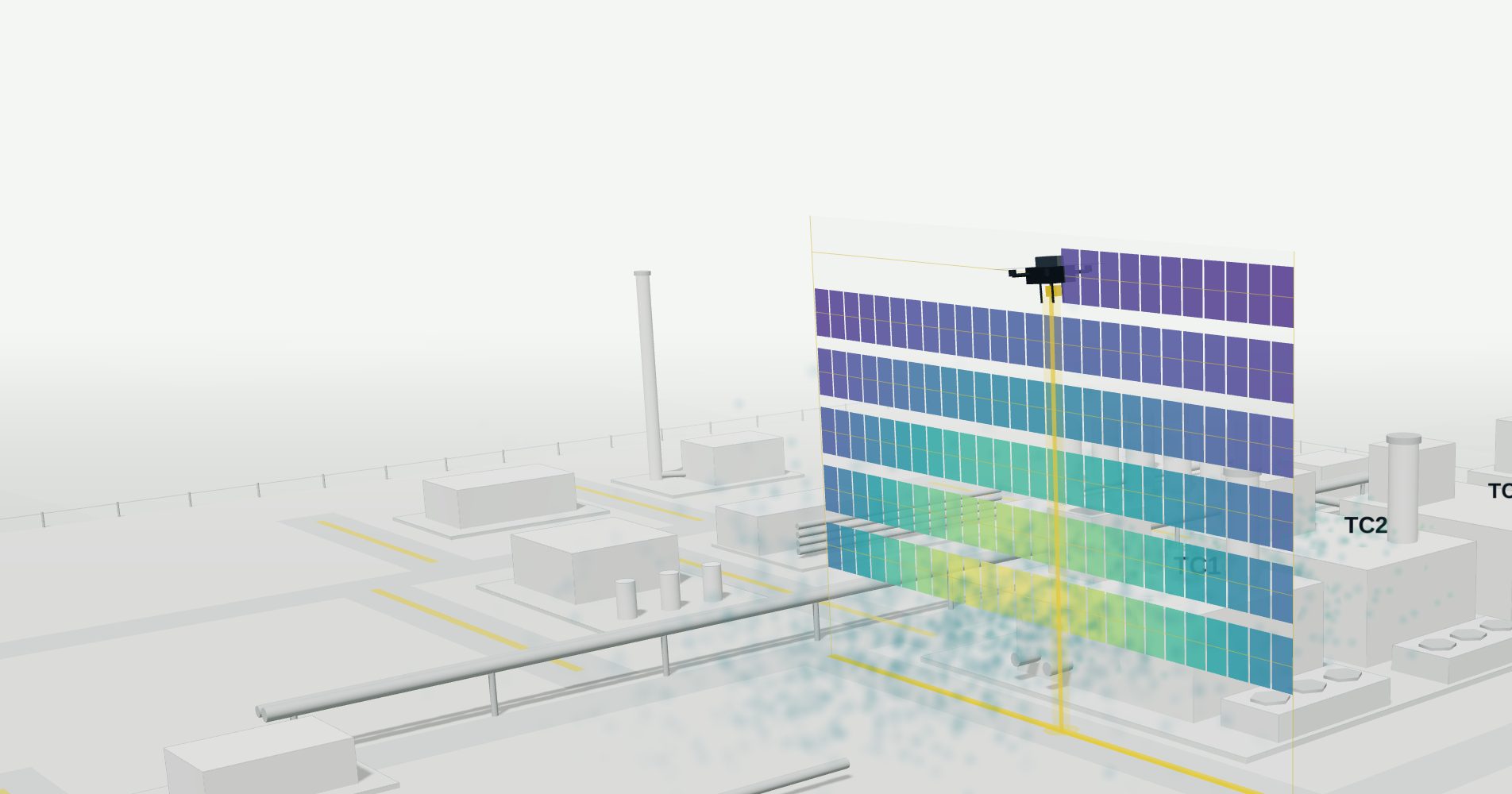
Drone survey of methane emissions at a gas compression station
Symbiotica flew a LASER FALCON downwind of eight plant sectors. From the ppm·m readings and on-site weather data, it estimated each sector's emission rate in kg/h.
- Site
- Natural gas compression station, operator not disclosed
- Survey and analysis
- Symbiotica S.r.l.
- Payload
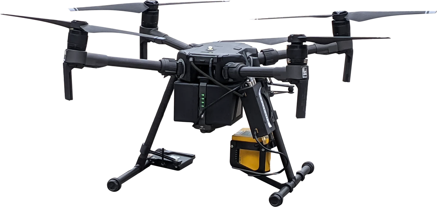
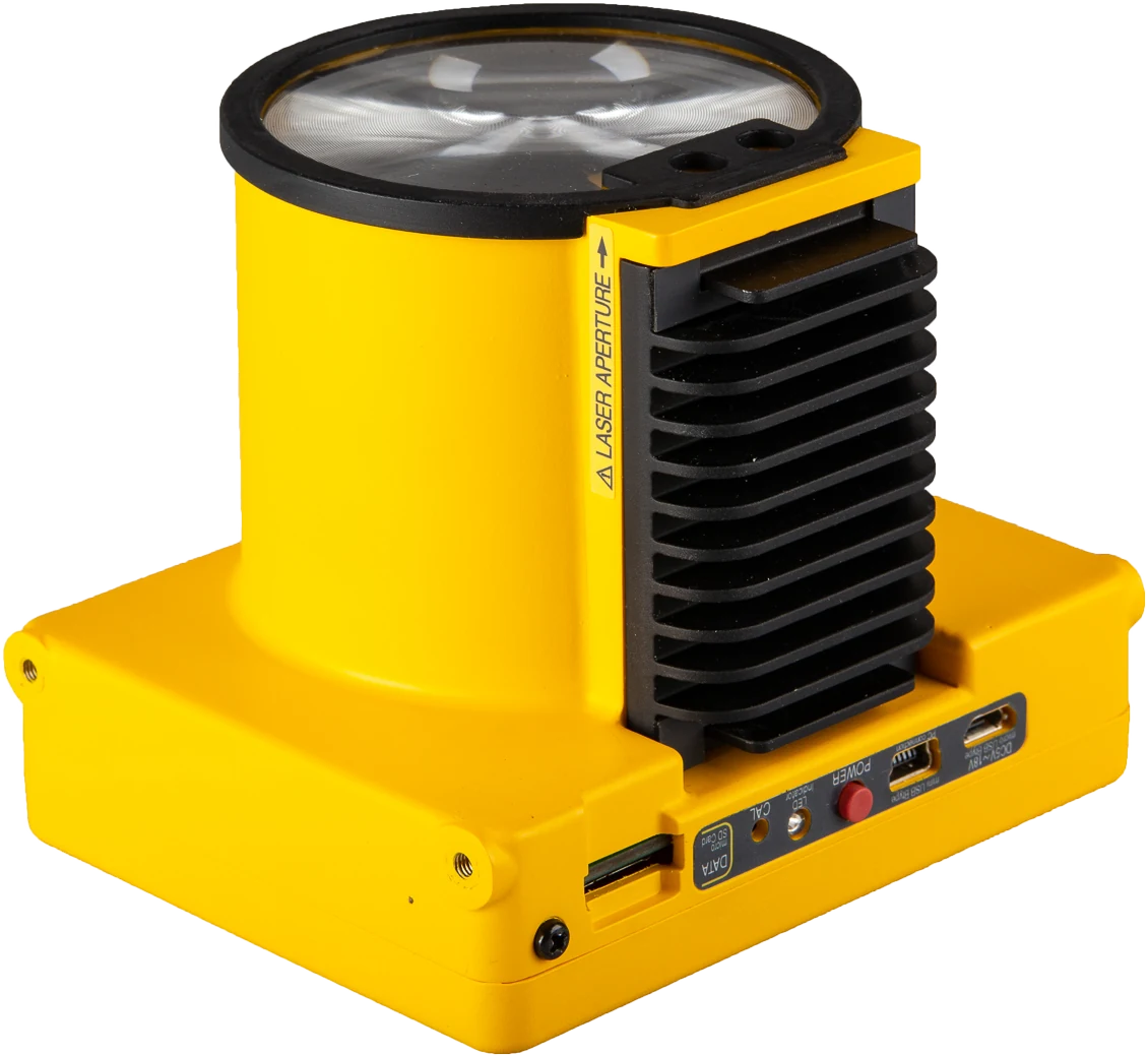
- LASER FALCON, open-path TDLAS, on a DJI M350 RTK
- Method
- UAV mass balance, transects from 10 to 35 m above ground
plant sectors, each measured from its own downwind flight line
transect heights, from 10 to 35 m above ground
of the estimated site emission rate came from the turbo-compressor area in Configuration 1 (about 86% in Configuration 2)
of the propagated uncertainty came from wind-speed variability, in every sector
The survey in 30 seconds
Station, flight lines, the laser reading, the measurement curtain and the result, reconstructed from the survey report.
What had to be measured
Symbiotica was commissioned to measure the methane released by the station, both for the whole site and for each of its process sectors. The sector boundaries were set by the client's staff.
The client asked for results in two operating configurations of the four turbo-compressor units. The measurements covered most of the station area. Flight paths followed the internal road network, so the drone never flew over above-ground plant structures.
| Unit | Configuration 1 | Configuration 2 |
|---|---|---|
| TC1 | Depressurised | Depressurised |
| TC2 | Compressing | Depressurised |
| TC3 | Compressing | Compressing |
| TC4 | Depressurised | Depressurised |
What was flown
Swipe sideways to see the whole diagram.
| Laser sensor | LASER FALCON, open-path tunable diode laser absorption spectroscopy (TDLAS). Wavelength 1.65 µm, pulses at 10 Hz, output in ppm·m, detection limit 1 ppm·m |
|---|---|
| Carrier | DJI M350 quadcopter with RTK positioning and a carbon-fibre frame, adapted for monitoring work: lighter components for longer endurance and custom brackets for the sensor |
| Height above ground | Radar altimeter |
| Positioning | RTK, centimetre-level. Used to follow the planned track and to georeference every reading |
| Ground station | Laptop connected to the remote controller. Sensor operation automated and monitored in real time; data logged both on the sensor and on the laptop |
| Weather station | Cup anemometer and wind vane at 2 m, air temperature and pressure, sampled at 2 Hz |

What a ppm·m reading is
The sensor sends a laser beam at a methane absorption wavelength down to the ground and measures how much of it is absorbed on the way. The result is the amount of methane along the whole optical path, expressed in ppm·m: concentration multiplied by path length.
A single reading says how much methane the beam crossed, not where along the path it was. In the example on the right both drones fly at 5 m over a uniform 2 ppm background. Drone A crosses a dense layer near the ground and reads 160 ppm·m. Drone B crosses a weaker, higher layer and reads 40 ppm·m.
The example is simplified: background is taken as uniform, and each plume layer is 1 m deep.
How the flights were run
The steps below follow the survey workflow described in the report.
Wind first
A weather station was set up during a preliminary walk-round, then moved next to the planned flight lines, away from vegetation, buildings and other obstacles that could distort the airflow.
Lines downwind of each sector
With the prevailing wind known, a flight line was placed downwind of each sector to intercept its plume. Flights started only after checking that nobody was in the overflight area.
A vertical curtain of transects
Each mission repeated the same horizontal track at progressively greater heights; in this survey the transects were flown between 10 and 35 m above ground. One transect took less than two minutes. Missions were planned around battery endurance so the aircraft could always return safely.
Check every flight
If concentrations were still high at the side or top edge of the scanned plane, the domain was widened and flown again. A spatio-temporal filter removed false readings caused by bright surfaces and by abrupt changes between surface types. A mission was repeated when its data were not representative.
From a reading to an emission rate
The emission rate of each sector was estimated with a Lagrangian mass balance: methane carried by the wind through the vertical plane of transects downwind of the source.
Schematic of the integration over height.
-
Convert the reading to mass
Ideal-gas conversion with the measured pressure P and temperature T; 16.04 g/mol is the molar mass of methane. The report puts the uncertainty from humidity below 1%, so the water-vapour term can be omitted when humidity is not measured.
-
Subtract the background
Background was taken as the 25th percentile of each flight's readings, after dividing them by the optical path length. Over large areas, where background points far outnumber plume points, the mode can be used instead.
-
Wind at every height
Logarithmic wind profile scaled from the 2 m station, with a stability correction Ψm based on the Monin–Obukhov length L and the surface roughness length z0.
-
Integrate over the plane
θ is the angle between wind and flight line, so only the wind component across the line carries gas through the plane. The subscripts d and b mark downwind and background values at height z for scan i.
-
Propagate the uncertainty
Wind speed and direction terms include the instrument uncertainty and the temporal variability (1σ). The concentration and position terms include instrument uncertainty only. Background drift within a transect was neglected, since one transect took under two minutes.
Eight sectors, eight flight lines
The site was divided into functional areas along the stages of gas treatment and compression. Each was measured from its own line on the downwind side, flown along the site roads.
Swipe sideways to see the whole plan.
| Sector | Flights | Discarded | Uncertainty, kg/h | |
|---|---|---|---|---|
| Config. 1 | Config. 2 | |||
| Site total, linear sum | 24 | 2 | ± 1.77 | ± 1.27 |
| Quadratic sum, for comparison | ≈ ± 1.51 | ≈ ± 1.06 | ||
Flight counts are for Configuration 1. In Configuration 2 the turbo-compressor area and the vent were flown again; the sectors marked * were carried over from Configuration 1.
Two sessions, two wind regimes
Wind is the main input of a mass balance, so it was recorded throughout. In the first session the flow came from the south-west with moderate variability. The second session had light wind with a wide spread of directions; the report notes that at such low speeds the gas is carried slowly through the plane, which makes the plume harder to capture.
Histograms redrawn from Figs. 6, 7, 17 and 18; the vertical axis is frequency, as in the report.
| Parameter | Configuration 1 | Configuration 2 |
|---|---|---|
| Wind speed, mean (median) | 2.53 m/s (2.60) | 1.04 m/s (1.10) |
| Wind speed, range | 0.00 to 5.70 m/s | 0.00 to 2.10 m/s |
| Wind speed, standard deviation | 0.98 m/s | 0.36 m/s |
| Wind direction, mean (median) | 214° (214°) | 231° (235°) |
| Wind direction, standard deviation | 40° | 80° |
| Air temperature, mean (range) | 20.9 °C (16.9 to 23.5) | 18.9 °C (16.9 to 20.8) |
| Pressure, mean (range) | 1009 hPa (1008 to 1013) | 1012 hPa (1012 to 1013) |
Where the methane came from
In both configurations the turbo-compressor area was the main source. The absolute emission rates are not disclosed; the shares and uncertainty bands below are as reported.
Why the totals use a linear sum
Sectors measured at the same time share the same wind, atmospheric stability and turbulence, and the same instrument response during altitude changes. Their errors cannot be treated as independent values that partly cancel out; they may be correlated. The report therefore adds the uncertainties of all sectors linearly, including those measured separately, a conservative worst case that assumes all deviations go in the same direction. Quadratic addition would give about ± 1.51 kg/h for Configuration 1 and ± 1.06 kg/h for Configuration 2.
Where the uncertainty came from
The uncertainty of each sector was split into its four inputs. The pattern was the same in every sector and in both configurations.
Swipe sideways to see the whole chart.
About 98% of the uncertainty came from wind-speed variability and about 1.5 to 2% from wind direction. The position term was 0.02 to 0.04%, and the ppm·m reading itself contributed less than 0.01%.
Read for this procedure, the result was limited by the wind input, not by the ppm·m reading. Steadier wind during the flights, or a wind measurement closer to the plane, would narrow it more than a more precise concentration reading would. This is our reading of the tables, not a conclusion stated in the report.
Two caveats. The concentration and position terms include only the stated instrument uncertainty of the sensors. And these shares describe this survey, its procedure and its weather; they should not be read as general figures for the method.
High concentration is not the same as high emission
The report also groups the readings into three classes of path-integrated concentration. In Configuration 1 the highest mean value in the top class, above 500 ppm·m, was recorded for GAME C. Yet the mass balance attributed about 85% of the site emission rate to the turbo-compressor area.
A reading depends on how much methane the beam crosses at that moment. An emission rate also needs the wind across the line and the whole plume cross-section, which is why the survey flew a full curtain of transects for every sector.
Scope of the results
- The results apply to this site, these two operating configurations and the weather on the survey dates. They are not general emission factors.
- The sector boundaries were set by the client, and each sector's rate refers to the area upwind of its flight line. The flight lines covered most of the station area, not all of it.
- In Configuration 2 only the turbo-compressor area and the vent were re-flown; the other sectors use Configuration 1 values, so the Configuration 2 total combines two survey sessions.
- Flights affected by false detections or unfavourable wind were excluded by the filtering algorithm: two of 24 in Configuration 1.
- Figures on this page are redrawn from the survey report. Where a figure and a table of the report differ, the table value is used. Animations are schematic.
Planning a methane quantification survey?
We can discuss sensor choice, mounting and flight planning for your site.
Credits
Survey, data processing and technical report: Symbiotica S.r.l., Taranto, an accredited spin-off of the University of Bari Aldo Moro.
Laser methane sensor: LASER FALCON by Pergam.
Using Pergam equipment in the field? We publish client case studies with a link to the client's website. Write to info@pergamitaly.eu.